How Should Productivity Be Used to Forecast Remaining Labour in Construction?

Same numbers, four forecasts

Here is what the four most obvious answers do to the estimate at completion. The project is synthetic — no real job, no employer data — and the numbers were picked to keep the arithmetic clean.

Figure 1

Scroll horizontally to read the full figure →

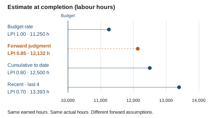
Roughly 2,100 hours separate the top and bottom of that list — a fifth of the original budget — and not one hour of it is measurement error. The earned hours, the actual hours and the remaining work are identical in all four rows. The only thing that changed is the answer to a question that often never gets asked out loud: what productivity do we expect for the work that is left?

That question sits inside every remaining-labour figure, whether anyone chose the answer or inherited it from whichever column the cost report already had. This article is about how I would answer it — on this project, at this data date — and how I would write the answer down so that it can be checked next cycle.

One thing to say before the theory arrives: there is not much theory. The arithmetic is three lines. The work is in the judgment.

What actually happened — and why

Cumulative 0.80 sounds like a description of the project. It is an average. Figure 2 is the history that produced it.

Figure 2

Scroll horizontally to read the full figure →

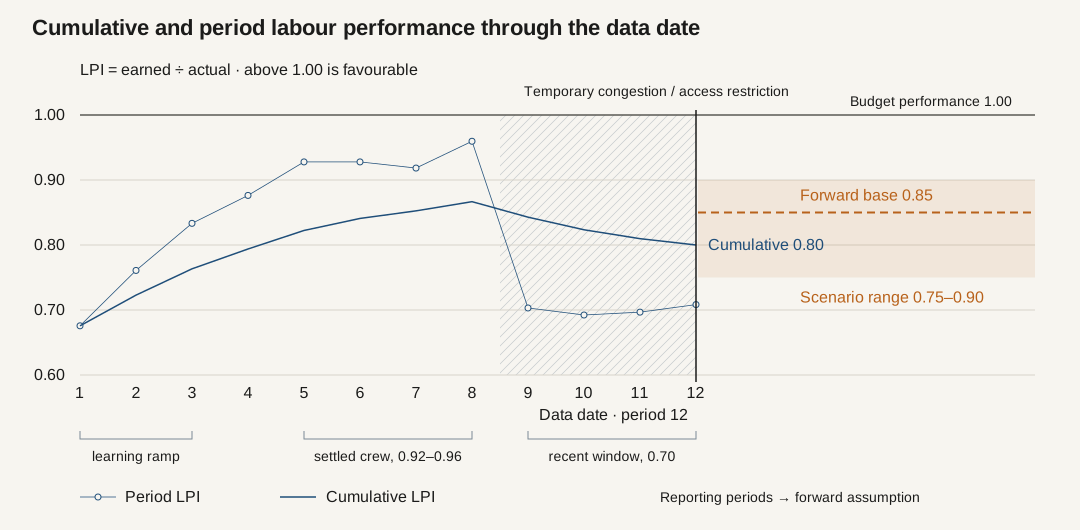
Read it left to right. Three periods of learning, then one transition period. Four periods where the crew, once settled, was close to budget performance. Then four periods at 0.70, coinciding with congestion and a temporary access restriction in the current area. The cumulative line blends all three into one number that describes none of them.

So the first question at a forecast review is not “what is the productivity?” It is “why did it change, and will that reason still be there?” There are really three possible answers, and established earned-value guidance already sorts forecasting formulas by them: when the current variance is unusual, forecast the rest at the budget rate; when it is the normal state of the project, apply the observed performance to the rest; and when the original estimate was wrong, stop applying factors and re-estimate the remaining work.¹ I read “unusual” as roughly nonrecurring and “normal” as roughly expected to continue — that is my interpretation of the wording, not theirs — but the point stands: choosing a rate is a diagnosis before it is a calculation.

On this project, the recent decline looks mostly temporary. The access restriction has an end date; the congestion goes with it. But not entirely: the remaining work mix is somewhat harder than the estimate assumed, and that will still be true after the restriction lifts. And on the third possibility — was the estimate simply wrong? — the settled-crew phase at 0.92–0.96 suggests the budget rate was not disconnected from what this crew could do, although they never actually reached 1.00. The evidence argues against a defective estimate without proving the rate was achievable.

Three reference points, one decision

When I am deciding what to assume, I find it useful to lay four numbers side by side. Three of them are evidence about the past. One is a decision about the future.

Figure 3

Scroll horizontally to read the full figure →

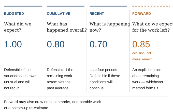
There is nothing new in the first three. Any earned-value text shows them, and every estimate-to-complete formula picks one or blends them. The reason for setting them out together is the fourth column: it can stay unwritten, inherited from whichever of the other three the reporting system defaults to, unless someone deliberately makes it a choice.

Two cautions that matter in practice. “Recent” is not a number until you say which window — the last period, the last four, the last fifth of earned hours all answer differently on a project whose performance is moving, and none of them is an industry-standard rule. In this example I use the last four periods, as an analytical choice. And the forward number does not have to come from a factor at all. If the remaining work is different enough, a bottom-up re-estimate by the people who will build it is often the more honest instrument. The choice about future performance is still in there — it is in the rates and crew assumptions the estimate uses — it just arrives from the field upward instead of the history forward.

What changes for the work that’s left

This is the question most easily skipped, and the one that most often moves the answer away from all three reference points. I split it in two, because the halves are different kinds of adjustment and get confused when they are mixed.

How much work remains? First separate quantity from productivity. If the scope grew, add the work — more earned hours to be credited — and don’t hide it inside a rate. Folding quantity growth into a productivity factor is how a scope problem gets misdiagnosed as a crew problem, or the reverse. On this project, remaining quantities and scope are unchanged, so the remaining earned hours stay at 5,000.

Under what conditions? Then ask whether the remaining work will be done under the conditions that produced the history. Table 1 is the list I work through. It is my synthesis, not a standard; that productivity is condition-sensitive is well supported — an electrical-contractor study built on 145 North American projects treats it that way, and estimating labour units are graded for normal, difficult and very difficult installation conditions⁴⁵ — but I am deliberately not quoting percentages. The public evidence I have does not support a specific loss for congestion or access, and any figure here would be invented.

Condition	Why it matters	Possible direction
Work mix	The rest may be a different blend of items than what’s done — each with its own budgeted rate	Either; often unfavourable late in a scope
Access	Scaffold, hoists, permits and other trades’ handovers decide how much workfront is usable	Either; improvement is often expected and often late
Sequence	Working out of planned order costs re-mobilisation and rework	Unfavourable when disrupted
Congestion and stacking	More crews in the same space than the estimate assumed	Unfavourable
Constraints	Design holds, RFIs, inspections, shutdown windows	Unfavourable while open
Crew	Continuity, size, skill mix, overtime, supervision; learning on repetitive work	Favourable with a continuing crew on repeating work; unfavourable with turnover or sustained overtime
Field conditions	Weather, temperature, logistics, travel to the work	Either
Material and equipment	Waiting converts crew time into idle time	Unfavourable when late

Scroll horizontally for all columns →

Source: Author's synthesis; directions are qualitative and situation-dependent.

Supporting condition evidence.⁴⁵

For this project: the access restriction ends and the workfront should open; the same core crew continues and may still be learning; the remaining mix is harder than estimated; materials are assumed stable. That is the whole inventory. The act of writing it down is what prompts the useful question — is the access date actually confirmed, or is it just in the look-ahead?

Three questions, in order

Put the diagnosis and the forward inventory together and you get the structure I use at a forecast review. I want to be plain about what it is: a working structure, close to ordinary variance analysis, not a validated method. I expect to revise it.

Figure 4

Scroll horizontally to read the full figure →

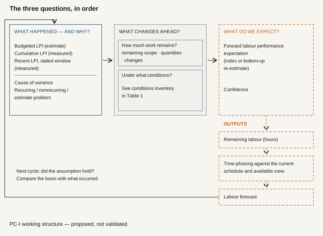
What happened — and why? Measured performance — budgeted, cumulative, and over a stated recent window. The cause. Whether it is recurring, nonrecurring, or an estimate problem.

What changes ahead? How much work remains, and under what conditions.

What do we expect? The forward performance expectation for the remaining work — as an index or a bottom-up estimate — and how confident we are.

The order is the point. Choose the rate first and the inventory becomes justification. Read the history first, then the conditions, and the rate falls out. From the decision come three outputs, not three more questions: the remaining hours; those hours placed in time against the schedule and the crew that will really be available; and the labour forecast that goes to whoever plans crews and cash. Then the loop closes: at the next data date, the first thing to check is whether last cycle’s expectation held.

Choosing 0.85 — and why not 0.80 or 0.70

Here is the reasoning laid out for this project. It is a board, not a calculation.

Figure 5

Scroll horizontally to read the full figure →

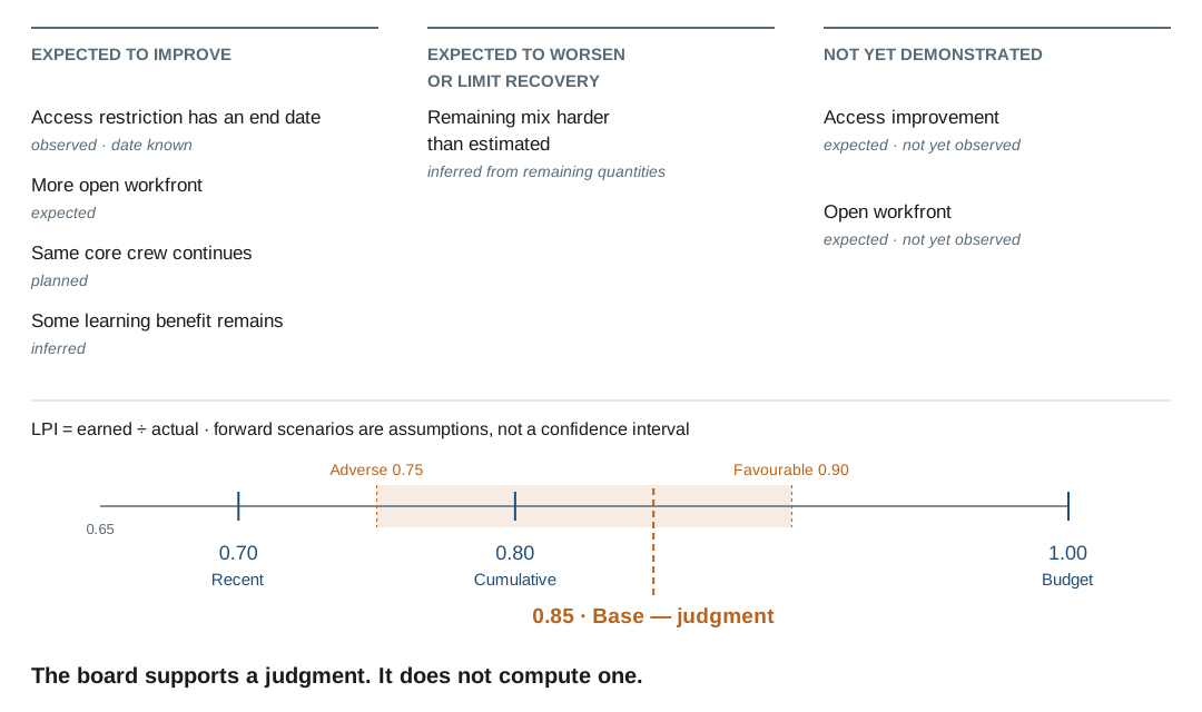
My base case is 0.85. Better than the congested window, because the restriction is ending and the workfront should open. Worse than the settled-crew phase, because the remaining mix is harder and the access improvement is expected rather than demonstrated. It is a judgment consistent with the board, not a number derived from it — another controls lead reading the same board could reasonably land at 0.80 or 0.88, and the right response to that is to write both rationales down, not to pretend one of them is arithmetic.

The arithmetic, once: 5,000 remaining earned hours ÷ 0.85 ≈ 5,900 hours to complete; add the 6,250 already spent, and the estimate at completion is about 12,100 hours.

The scenarios bracket the two conditions the board marks as not yet demonstrated. Favourable (0.90) assumes access opens on time and the learning is real. Adverse (0.75) assumes access stays tight and the harder mix bites. I am not claiming a range is more accurate than a point; the evidence I have supports looking at more than one forecast,⁶ not that scenarios win.

Assumption	LPI	ETC (h)	EAC (h)	EAC ÷ budget
Budget rate — variance treated as nonrecurring	1.00	5,000	11,250	1.13
Cumulative to date	0.80	6,250	12,500	1.25
Recent — last four periods	0.70	7,143	13,393	1.34
Forward — base	0.85	5,882	12,132	1.21
Forward — favourable	0.90	5,556	11,806	1.18
Forward — adverse	0.75	6,667	12,917	1.29

Scroll horizontally for all columns →

Source: Author's synthetic example. Budget 10,000 h; earned 5,000 h; actual 6,250 h; remaining earned 5,000 h. LPI = earned ÷ actual. Values rounded to whole hours; prose uses coarser rounding.

Then I write it down. Not as a governance form — as a note a colleague, a client’s controls team, or I myself three months later can read and argue with.

Two things about the note. The trigger is deliberately not a number: the reasons for 0.85 were the restriction ending and the workfront opening, so the trigger is whether they did. And the note is what closes the loop. When the next period’s actuals arrive, the first check is not the new cumulative index but whether the basis held — did access open, did the mix bite, was it the same crew? I have no evidence that writing the assumption down makes forecasts more accurate. What it does is make forecast error attributable, and attributable error is the only kind you can learn from.

The two habits I watch for in myself: anchoring on the budget rate because it is the number everyone signed, and treating an access date as a fact because it is in the look-ahead.

Does the research give us a winning number?

No — and it is worth knowing exactly how much it does give.

Construction research supports using actual performance as an input to the forecast, but it does not hand us one universally better rate. A 1994 study of 22 masonry projects found that a factor model using actual performance forecast within ±5% on average with only 5% of the work done, with a spread of ±25% based on standard deviation; a much simpler method — hours to date divided by percent complete — was just as accurate on average, but with an error range about half again as wide.⁷ That is one trade, one sample, three decades ago, and I would not carry it to other trades without more. A 2024 study tested 71 performance factors across 65 real projects and found no clear winner among the progress-based factors it examined; the gains it did find were dataset-specific and modest, and its advice was to look at forecasts from several factors rather than trust one.⁶ That study is about cost and duration, not labour hours, so it validates nothing here directly.

What I take from both: feeding measured performance into the forecast is better than ignoring it; the spread of possible outcomes stays wide; and the search for the one correct factor is not going to end in a formula. If no single factor wins across 65 projects, the choice is a judgment — which is the case for writing it down.

Hours are not yet a forecast

About 5,900 hours answers “how many.” It does not answer “when,” “by whom,” or “can the site absorb them.” A labour forecast — the crew curve someone will actually staff to — needs those hours placed in time against the current schedule, under the crew, calendar, access and material constraints that really exist.

That is a separate step, and it is where the resource-loaded schedule comes in. It is easy to say something sharp and wrong here, so: a resource-loaded schedule is not “just a plan.” A current schedule by definition carries actual progress plus a forecast going forward,³ the GAO’s schedule-assessment practice expects an update to refresh remaining effort and resource use rather than only dates,⁸ and the scheduling tools let you re-estimate remaining future-period units when work departs from plan.⁹ A properly maintained resource-loaded schedule can carry a perfectly credible labour forecast. The question is whether, in the last update, someone actually re-estimated the remaining units in light of the three questions above — or whether the tool spread the original planned units across new dates and called it a forecast. When a resource-loaded schedule becomes a trustworthy labour forecast is the next piece in this series.

Five questions I would take into the next forecast review

1. What did we actually earn for the hours we spent — overall, and over the last few periods?
2. Why did performance change, and is that cause still going to be there?
3. How much work really remains — has the scope grown, and are we adding it as work rather than hiding it in a rate?
4. Which conditions will be different for the remaining work — access, mix, sequence, crew, materials?
5. What forward assumption are we using, what did we reject, and what would make us change it?

What remains open is real. The research doesn’t tell us which window or adjustment forecasts remaining trade labour best, whether that changes by trade or phase, or whether writing the reasoning down improves accuracy rather than just explanation. I intend to test that on a synthetic project with controlled disruptions and publish what breaks.

And I would like to be argued with. If your schedule or cost system updates remaining hours, do you know whether a person re-estimated them or the tool recalculated them? When observed productivity differs from the estimate, what test tells you the variance is recurring? And if you think one of the three reference points should be carried forward by default, I want to hear the conditions under which you have seen that work.

Key takeaways

Open questions

• When your system is updated, are remaining labour hours recalculated by the tool, re-estimated by a person, or left as planned less actual — and how can you tell?
• What test do you use to decide whether a productivity variance is recurring, nonrecurring, or a sign the estimate was wrong?
• Do you keep forecast snapshots and compare them with later actual labour — at which horizons, with what error measures?

References

1. Prasad, V., Rajkumar, P. and Rastogi, S. C. (2006). Managing firmed fixed price projects using EVM: a case study. PMI Global Congress — Asia Pacific, Bangkok. “Broad understanding of EVM,” Basic Forecast Metric table, EAC row. A PMI-published conference case-study paper (IT services), not a PMI standard; the reading of “unusual” as nonrecurring and “normal” as continuing is the author’s. Source ↩

2. McLin, M. (2019). Productivity Tracking in the HVAC and Sheet Metal Industry. New Horizons Foundation, via SMACNA. “Productivity,” printed p. 33 (example: 90 actual ÷ 80 earned = 1.125). Source ↩

3. AACE International (2026). Recommended Practice 10S-90: Cost Engineering Terminology. Entries for “Estimate to Complete,” “Forecast,” “Current Schedule,” “Labor Productivity” and “Labor Productivity Factor” (printed p. 87). Source ↩ ↩²

4. Hanna, A. (2018). Factors Affecting Labor Productivity for Electrical Contractors. ELECTRI International, report F3418, September 2018. Project count as described on the publisher’s page. Source ↩ ↩²

5. NECA (2023). Manual of Labor Units, 2023–2024 edition. Installation-condition sections. Source ↩ ↩²

6. Ottaviani, F. M., De Marco, A., Narbaev, T. and Rebuglio, M. (2024). “Improving Project Estimates at Completion through Progress-Based Performance Factors.” Buildings, 14(3), 643. 71 factors; 65 projects; 1,235 observations interpolated at 5% progress steps; dataset-specific gains ranked precision, timeliness, accuracy; cost and duration forecasting. Source ↩ ↩²

7. Thomas, H. R. and Sakarcan, A. S. (1994). “Forecasting Labor Productivity Using Factor Model.” Journal of Construction Engineering and Management, 120(1), 228–239. Figures from the published abstract; the ±25% is a range based on standard deviation, not a prediction interval. Source ↩

8. U.S. Government Accountability Office (2015). GAO Schedule Assessment Guide, GAO-16-89G, 22 December 2015. Best Practice 9, updating the schedule with actual progress and logic. Source ↩

9. Oracle (2026). Primavera P6 Professional User Guide — Future period bucket planning. Vendor documentation, cited for capability only. Source ↩